User’s data#

Forest cover change map#

You can use your own forest cover change map with the plugin. To do so, prepare a raster file and select it with the Forest data source argument in the Get variables tab of the plugin. The raster file will be automatically copied in the data_raw folder of the working directory and renamed forest_src.tif. The raster file should have the following characteristics:

It must be a multiple band raster file with each band representing the forest cover at one date.
Bands must be ordered (first band for t, second band for t+1, etc.).
Raster should only have two values: 1 for forest pixels and 0 for non-forest pixels (the raster can thus be of type Byte).
No-data value is not important here. It can be set to 0 or 255 for example.
The raster file should be projected in the coordinate reference system of the project (see argument projection EPSG code).
The raster must cover at least all the area of the jurisdiction.
Years specified in the Years argument should correspond to the years used for the forest cover change raster file.

Warning

It is much better if the raster is bigger than the jurisdiction (e.g. buffer of 10 km) to reduce edge effects when computing distances to forest edge for example.

While executing the Get variables step, this raster will be used as the forest data source and all the forest variables (forest cover change and distance to forest edge at the different dates) will be computed from this data.

You can create this multiple band raster using the QGIS tool Merge available in Raster > Miscellaneous.

Area of interest#

You can specify your area of interest when using the plugin. To do so, prepare a vector file and select it with the Area Of Interest argument in the Get variables tab of the plugin. The vector file will be automatically copied in the data_raw folder of the working directory and renamed aoi_latlon.gpkg. The vector file should have the following characteristics:

It must be in lat/lon (i.e. unprojected with EPSG code 4326).
It must have two layers named aoi for the jurisdiction and subj for the subjurisdictions.

More details on how to obtain such vector file in QGIS are available in the article untitled Subnational jurisdictions.

Additional explicative variables#

Prepare the raster files#

To use different or additional explicative variables for the statistical models, prepare the corresponding raster files in the data folder of the working directory. These additional raster files should have the following characteristics:

They should cover at least all the area of the jurisdiction.
They should be in the projection of the project.
Resolution should be as close as possible to the forest cover raster resolution.

If some of these variables are changing with time, then create several rasters for t1, t2, and t3.

Copy files in the right folders#

Raster files of explanatory variables must be copied in the folders data_calibration, data_validation, data_historical, and data_forecast of the working directory. These directories are used to access both the forest cover change and the explanatory variables for modelling and predicting the deforestation risk for the different periods.

If using variables changing with time, prepare three rasters variable_t1.tif, variable_t2.tif, and variable_t3.tif. Copy these rasters in the corresponding folders and change the raster names to variable.tif. It is important that the different rasters have the same name variable.tif in the different folders so that the algorithm understands it refers to the same variable:

In the data_calibration and data_historical folders (for which we use variables at t1), the file variable.tif should be a copy of the file variable_t1.tif.
In the data_validation folder (for which we use variables at t2), the file variable.tif should be a copy of the file variable_t2.tif.
In the data_forecast folder (for which we use variables at t3), the file variable.tif should be a copy of the file variable_t3.tif.

Create symbolic links to save space on disk (optional)#

To avoid copying the same data at several places on disk, you can create symbolic links in each of the folders data_calibration, data_validation, data_historical, and data_forecast. Symbolic links could point to rasters in the data folder for example.

If using changing variables with time, then use the same file name (e.g. variable.tif) for symbolic links in the four data_* folders but pointing to different files variable_t*.tif in the data folder. For example:

In the data_calibration and data_historical folders (for which we use variables at t1), the file variable.tif should point to the file variable_t1.tif in the data folder.
In the data_validation folder (for which we use variables at t2), the file variable.tif should point to the file variable_t2.tif in the data folder.
In the data_forecast folder (for which we use variables at t3), the file variable.tif should point to the file variable_t3.tif in the data folder.

To create symbolic links in Windows, use the command mklink. To be able to create symbolic links, the Developer Mode must be activated on your computer.

# Create a symbolic link in Windows
mklink "C:\Users\me\deforisk\MTQ\data_calibration\variable.tif" "C:\Users\me\deforisk\MTQ\data\variable_t1.tif"

Use these variables in the formula for the statistical models#

If raster variable.tif was added to the list of explanatory variables, then add its name variable to the list of variables names for the FAR statistical models, see detail here.

No internet connexion needed#

Provide you own data#

If you use your own data with the deforisk plugin, there is no need for an internet connexion. You just have to provide:

The forest cover change data as a multiband raster file (see Forest cover change map section).
The area of interest as a vector file (see Area of interest section).
The raster files of explanatory variables in the folders data_calibration, data_validation, data_historical, and data_forecast of the working directory (see Copy files section).

Also, you don’t need credentials to download data from Google Earth Engine or the World Database on Protected Area. Parameters Earth Engine access and WDPA access can be left empty. Button Only compute forest variables must be checked.

A simple approach with only forest variables#

Distance to forest edge is usually the most important variable in determining the spatial deforestation risk. It can be useful to compare and evaluate models using only this explanatory variable. To do so, you just have to:

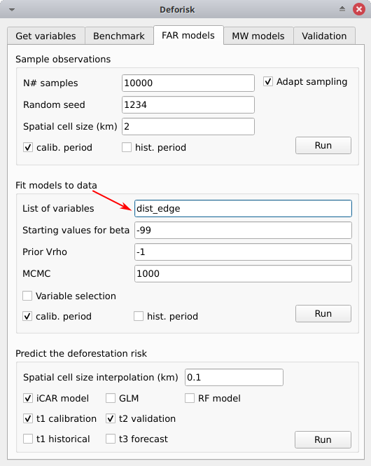
Check the button Only compute forest variables.
Specify ’dist_edge’ in the List of variables for FAR models.

Distance to forest edge is directly computed from the forest cover change raster file and you don’t have to provide any other additional explanatory variables.

A simple example with no internet connexion#

As an example based on Martinique, you can avoid using an internet connexion and use simple deforestation models based only on distance to forest edge:

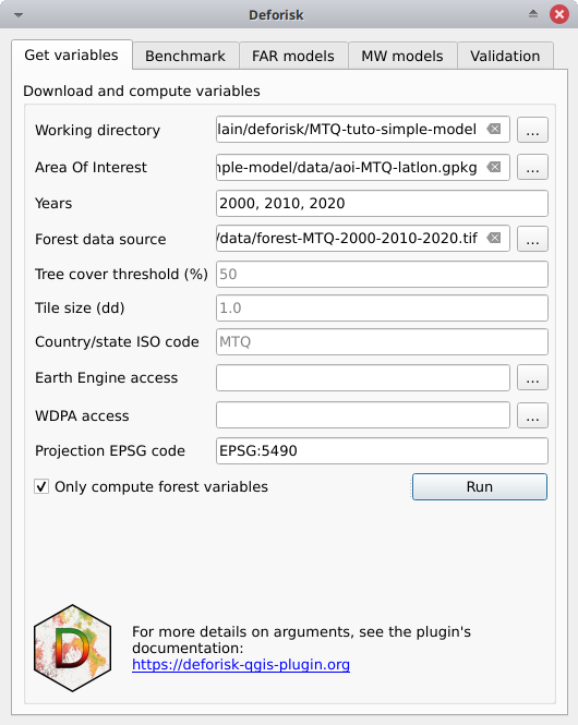
Create a working directory called for example MTQ-tuto-simple-model.
Create a data_user directory and copy files forest-MTQ-2000-2010-2020.tif and aoi-MTQ-latlon.gpkg in this directory.
Use these two files for arguments Area Of Interest and Forest data source in the Get variables tab.
Specify ’2000, 2010, 2020’ for Years.
Use ’EPSG:3490’ for Projection EPSG code.
Ensure Only compute forest variables is checked.
All other variables in the Get variables tab can be left empty.
Click Run in the Get variables tab to compute forest variables.

../_images/user-data-interface-variables.png

Specify only ’dist_edge’ in the List of variables for FAR models and run the models and the validation with the default parameters.